Matrix Decomposition

本文试图用最简洁清晰的语言解释各种矩阵分解，只记录矩阵分解的基础知识和过程，对性质和应用的讨论先挖个坑，下次再填

有关矩阵分解的知识可以参考这个

为什么要矩阵分解？为了更好的计算，降低计算复杂度

Definitions

Unitary matrix

Conjugate transpose

共轭转置 aka Hermitian transpose，计$A^H$为A的共轭转置（有时也写成$A^*$）

对实矩阵，${\displaystyle {\boldsymbol {A}}^{\mathrm {H} }={\boldsymbol {A}}^{\mathsf {T}}}$

对矩阵A，共轭转置后，每个元素的定义为

$${\displaystyle \left({\boldsymbol {A}}^{\mathrm {H} }\right)_{ij}={\overline {{\boldsymbol {A}}_{ji}}}}$$

比如矩阵A

$$ {\displaystyle {\boldsymbol {A}}={\begin{bmatrix}1&-2-i&5\\1+i&i&4-2i\end{bmatrix}}} $$

$$ {\displaystyle {\boldsymbol {A}}^{\mathsf {T}}={\begin{bmatrix}1&1+i\\-2-i&i\\5&4-2i\end{bmatrix}}} $$

$$ {\displaystyle {\boldsymbol {A}}^{\mathrm {H} }={\begin{bmatrix}1&1-i\\-2+i&-i\\5&4+2i\end{bmatrix}}} $$

酉矩阵的定义为，对于方阵U，满足如下性质，U*是共轭转置，I是单位阵

$$ {\displaystyle U^{*}U=UU^{*}=UU^{-1}=I} $$

酉矩阵的行列式绝对值为1，在特征空间中正交，当矩阵为实数阵时，就是正交矩阵（orthogonal matrix）

正交矩阵就是各列向量线性无关，是实数下的酉矩阵

Definite matrix

Definitions for real matrices

假设M是n阶实对称矩阵

$$ {\displaystyle M{\text{ positive-definite}}\quad \iff \quad \mathbf {x} ^{\textsf {T}}M\mathbf {x} >0{\text{ for all }}\mathbf {x} \in \mathbb {R} ^{n}\setminus \{\mathbf {0} \}} $$

$$ {\displaystyle M{\text{ positive semi-definite}}\quad \iff \quad \mathbf {x} ^{\textsf {T}}M\mathbf {x} \geq 0{\text{ for all }}\mathbf {x} \in \mathbb {R} ^{n}} $$

$$ {\displaystyle M{\text{ negative-definite}}\quad \iff \quad \mathbf {x} ^{\textsf {T}}M\mathbf {x} <0{\text{ for all }}\mathbf {x} \in \mathbb {R} ^{n}\setminus \{\mathbf {0} \}} $$

$$ {\displaystyle M{\text{ negative semi-definite}}\quad \iff \quad \mathbf {x} ^{\textsf {T}}M\mathbf {x} \leq 0{\text{ for all }}\mathbf {x} \in \mathbb {R} ^{n}} $$

Definitions for complex matrices

设M是n阶Hermite复矩阵

$$ {\displaystyle M{\text{ positive-definite}}\quad \iff \quad \mathbf {x} ^{*}M\mathbf {x} >0{\text{ for all }}\mathbf {x} \in \mathbb {C} ^{n}\setminus \{\mathbf {0} \}} $$

$$ {\displaystyle M{\text{ positive semi-definite}}\quad \iff \quad \mathbf {x} ^{*}M\mathbf {x} \geq 0{\text{ for all }}\mathbf {x} \in \mathbb {C} ^{n}} $$

$$ {\displaystyle M{\text{ negative-definite}}\quad \iff \quad \mathbf {x} ^{*}M\mathbf {x} <0{\text{ for all }}\mathbf {x} \in \mathbb {C} ^{n}\setminus \{\mathbf {0} \}} $$

$$ {\displaystyle M{\text{ negative semi-definite}}\quad \iff \quad \mathbf {x} ^{*}M\mathbf {x} \leq 0{\text{ for all }}\mathbf {x} \in \mathbb {C} ^{n}} $$

正定矩阵的几何意义参考此处

实际上$x^TAx$的形式表示二次型（有一个概念叫合同与之相关），而根据定义，正定矩阵表示对所有的非零解，它的值都是大于0的，这在空间上是一个开口向上的抛物面（三维），正定矩阵如果看做一种空间变换，就相当于把一块布的四个角往上提了

假设$y=x^TAx$，那么y>0，且y有最小值

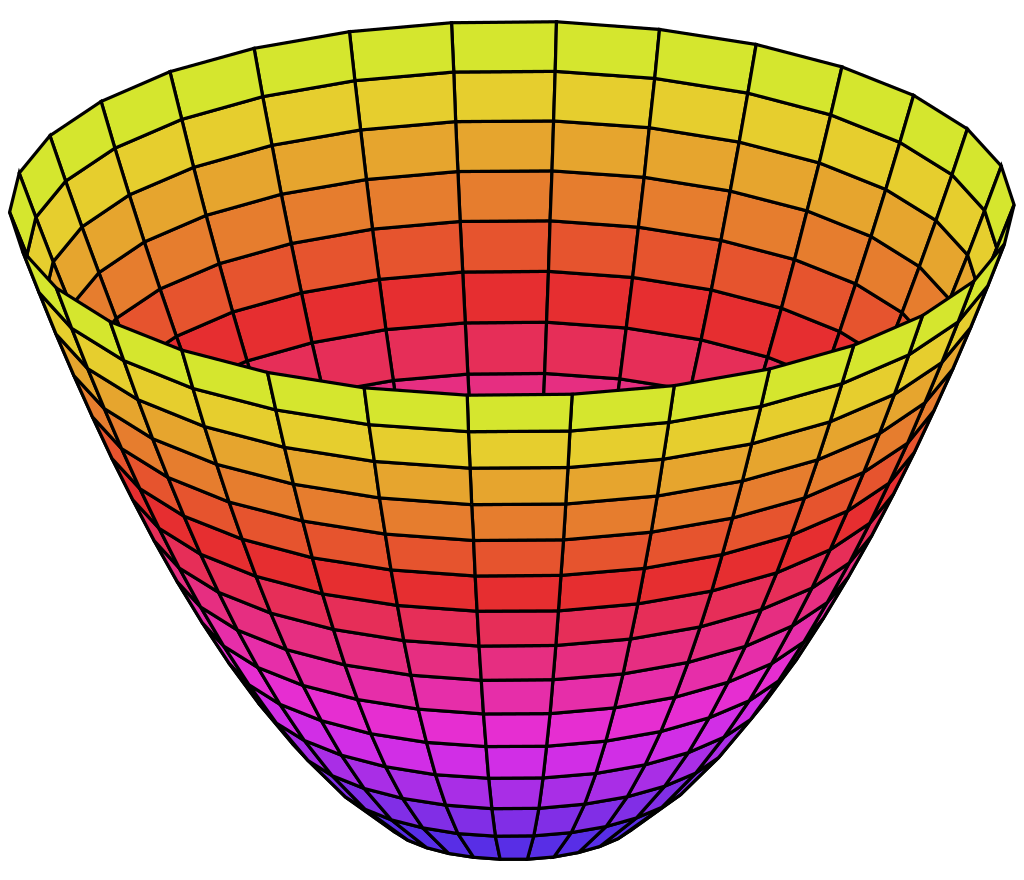
当我们求一个二次型的极值时，假设它是正定矩阵，那么一定有最小值（如上图），而根据泰勒公式，Hessian矩阵就是二次型的矩阵A，所以判断Hessian矩阵是不是正定矩阵就行

Example

单位阵是正定矩阵也是正半定矩阵

$$ {\displaystyle\mathbf{z}^{\textsf{T}}I\mathbf{z}={\begin{bmatrix}a&b\end{bmatrix}}{\begin{bmatrix}1&0\\0&1\end{bmatrix}}{\begin{bmatrix}a\\b\end{bmatrix}}=a^{2}+b^{2}.} $$

这个矩阵M也是正定矩阵

$$ {\displaystyle M={\begin{bmatrix}2&-1&0\\-1&2&-1\\0&-1&2\end{bmatrix}}} $$

$$ {\displaystyle {\begin{aligned}\mathbf {z} ^{\textsf {T}}M\mathbf {z} =\left(\mathbf {z} ^{\textsf {T}}M\right)\mathbf {z} &={\begin{bmatrix}(2a-b)&(-a+2b-c)&(-b+2c)\end{bmatrix}}{\begin{bmatrix}a\\b\\c\end{bmatrix}}\\&=(2a-b)a+(-a+2b-c)b+(-b+2c)c\\&=2a^{2}-ba-ab+2b^{2}-cb-bc+2c^{2}\\&=2a^{2}-2ab+2b^{2}-2bc+2c^{2}\\&=a^{2}+a^{2}-2ab+b^{2}+b^{2}-2bc+c^{2}+c^{2}\\&=a^{2}+(a-b)^{2}+(b-c)^{2}+c^{2}\end{aligned}}} $$

这个矩阵N不是正定矩阵

$$ {\displaystyle N={\begin{bmatrix}1&2\\2&1\end{bmatrix}}} $$

$$ {\displaystyle {\begin{bmatrix}-1&1\end{bmatrix}}N{\begin{bmatrix}-1&1\end{bmatrix}}^{\textsf {T}}=-2<0} $$

Eigenvalues

Type	Condition(iff all eigenvalues are)
positive definite	positive
positive semi-definite	non-negative
negative definite	negative
negative semi-definite	non-positive
indefinite	both positive and negative

Hermitian matrix

共轭转置为自身的方阵叫Hermite矩阵

$$ {\displaystyle A{\text{ Hermitian}}\quad \iff \quad a_{ij}={\overline {{a}_{ji}}}} $$

或者

$$ {\displaystyle A{\text{ Hermitian}}\quad \iff \quad A=A^{\mathsf {H}}} $$

Hermite矩阵的对角线必须为实数，如下就是一个Hermite矩阵，由此可见对称矩阵一定是Hermite矩阵

$$ {\displaystyle {\begin{bmatrix}0&a-ib&c-id\\a+ib&1&m-in\\c+id&m+in&2\end{bmatrix}}} $$

Eigenvalues and eigenvectors

此处可以去看3b1b的视频，讲解非常清晰

只有方阵才有特征值和特征向量

方阵的秩不小于它的非零特征值的个数

一个特征值可以有多个特征向量

在实数范围内，可能没有特征值和特征向量，但是在复数范围内，一定有，且有无穷多个特征向量

几何意义是：

方阵可以看作是对空间的一种线性变换，特征向量就是变化后方向保持不变的向量，特征值就是特征向量在变换后放缩的倍率。

行列式是平行四边形包围的面积，如果为负，就类似于平面翻转

Gram–Schmidt process

施密特正交法用于在欧氏空间中，给定线性无关向量组求标准正交基的过程

给定v，求e

$$ {\displaystyle \operatorname {proj} _{\mathbf {u} }(\mathbf {v} )={\frac {\langle \mathbf {u} ,\mathbf {v} \rangle }{\langle \mathbf {u} ,\mathbf {u} \rangle }}{\mathbf {u} }} $$

$$ {\displaystyle {\begin{aligned}\mathbf{u} _{1}&=\mathbf {v} _{1},&\mathbf {e} _{1}&={\frac {\mathbf {u} _{1}}{|\mathbf {u} _{1}|}}\\\mathbf {u} _{2}&=\mathbf {v} _{2}-\operatorname {proj} _{\mathbf {u} _{1}}(\mathbf {v} _{2}),&\mathbf {e} _{2}&={\frac {\mathbf {u} _{2}}{|\mathbf {u} _{2}|}}\\\mathbf {u} _{3}&=\mathbf {v} _{3}-\operatorname {proj} _{\mathbf {u} _{1}}(\mathbf {v} _{3})-\operatorname {proj} _{\mathbf {u} _{2}}(\mathbf {v} _{3}),&\mathbf {e} _{3}&={\frac {\mathbf {u} _{3}}{|\mathbf {u} _{3}|}}\\\mathbf {u} _{4}&=\mathbf {v} _{4}-\operatorname {proj} _{\mathbf {u} _{1}}(\mathbf {v} _{4})-\operatorname {proj} _{\mathbf {u} _{2}}(\mathbf {v} _{4})-\operatorname {proj} _{\mathbf {u} _{3}}(\mathbf {v} _{4}),&\mathbf {e} _{4}&={\mathbf {u} _{4} \over |\mathbf {u} _{4}|}\\&{}\ \ \vdots &&{}\ \ \vdots \\\mathbf {u} _{k}&=\mathbf {v} _{k}-\sum _{j=1}^{k-1}\operatorname {proj} _{\mathbf {u} _{j}}(\mathbf {v} _{k}),&\mathbf {e} _{k}&={\frac {\mathbf {u} _{k}}{|\mathbf {u} _{k}|}}\end{aligned}}} $$

Gaussian elimination

Introduction

高斯消元可以用来求线性方程组的解，矩阵的秩，方阵的行列式，可逆矩阵的逆等等。

高斯消元使用初等行变换（elementary row operations），使矩阵有更多的0元素

初等行变换有3种

• 交换两行
• 对某一行乘上任意非零数
• 将某一行的倍数加到另一行（减同理）

高斯消元首先将矩阵变成行阶梯形式（row echelon form），此时可以判断方程无解、有唯一解、无穷多解，然后再变成最简行阶梯形式（reduced row echelon form），此时可以求出具体的解，转化到最简行阶梯矩阵的过程又叫Gauss–Jordan elimination

首项系数（leading coefficients）是每一行的第一个非0数，比如下面红色的数

$$ \left[\begin{array}{cccc} 0 & \color{red}{2} & 1 & -1\\0 & 0 & \color{red}3 & 1\\0 & 0 & 0 & 0 \end{array}\right] $$

最简行阶梯形式就是首项系数为1，首项系数所在的每一列，除了它以外全是0

高斯消元的过程如下

$$ \left[\begin{array}{cccc} 1 & 3 & 1 & 9 \\1 & 1 & -1 & 1 \\3 & 11 & 5 & 35 \end{array}\right] \rightarrow\left[\begin{array}{cccc} 1 & 3 & 1 & 9 \\0 & -2 & -2 & -8 \\0 & 2 & 2 & 8 \end{array}\right] \rightarrow\left[\begin{array}{cccc} 1 & 3 & 1 & 9 \\0 & -2 & -2 & -8 \\0 & 0 & 0 & 0 \end{array}\right] \rightarrow\left[\begin{array}{cccc} 1 & 0 & -2 & -3 \\0 & 1 & 1 & 4 \\0 & 0 & 0 & 0 \end{array}\right] $$

Example

假设要求解的方程组为

$$ {\displaystyle {\begin{alignedat}{4}2x&{}+{}&y&{}-{}&z&{}={}&8&\qquad (L_{1})\\-3x&{}-{}&y&{}+{}&2z&{}={}&-11&\qquad (L_{2})\\-2x&{}+{}&y&{}+{}&2z&{}={}&-3&\qquad (L_{3})\end{alignedat}}} $$

高斯消元的过程如下

System of equations	Row operations	Augmented matrix
$${\displaystyle {\begin{alignedat}{4}2x&{}+{}&y&{}-{}&z&{}={}&8&\\-3x&{}-{}&y&{}+{}&2z&{}={}&-11&\\-2x&{}+{}&y&{}+{}&2z&{}={}&-3&\end{alignedat}}}$$		$${\displaystyle \left[{\begin{array}{rrr|r}2&1&-1&8\\-3&-1&2&-11\\-2&1&2&-3\end{array}}\right]}$$
$${\displaystyle {\begin{alignedat}{4}2x&{}+{}&y&{}-{}&z&{}={}&8&\\&&{\tfrac {1}{2}}y&{}+{}&{\tfrac {1}{2}}z&{}={}&1&\\&&2y&{}+{}&z&{}={}&5&\end{alignedat}}}$$	$${\displaystyle {\begin{aligned}L_{2}+{\tfrac {3}{2}}L_{1}&\to L_{2}\\L_{3}+L_{1}&\to L_{3}\end{aligned}}}$$	$${\displaystyle \left[{\begin{array}{rrr|r}2&1&-1&8\\0&{\frac {1}{2}}&{\frac {1}{2}}&1\\0&2&1&5\end{array}}\right]}$$
$${\displaystyle {\begin{alignedat}{4}2x&{}+{}&y&{}-{}&z&{}={}&8&\\&&{\tfrac {1}{2}}y&{}+{}&{\tfrac {1}{2}}z&{}={}&1&\\&&&&-z&{}={}&1&\end{alignedat}}}$$	$${\displaystyle L_{3}+-4L_{2}\to L_{3}}$$	$${\displaystyle \left[{\begin{array}{rrr|r}2&1&-1&8\\0&{\frac {1}{2}}&{\frac {1}{2}}&1\\0&0&-1&1\end{array}}\right]}$$
$${\displaystyle {\begin{alignedat}{4}2x&{}+{}&y&&&{}={}7&\\&&{\tfrac {1}{2}}y&&&{}={}{\tfrac {3}{2}}&\\&&&{}-{}&z&{}={}1&\end{alignedat}}}$$	$${\displaystyle {\begin{aligned}L_{2}+{\tfrac {1}{2}}L_{3}&\to L_{2}\\L_{1}-L_{3}&\to L_{1}\end{aligned}}}$$	$${\displaystyle \left[{\begin{array}{rrr|r}2&1&0&7\\0&{\frac {1}{2}}&0&{\frac {3}{2}}\\0&0&-1&1\end{array}}\right]}$$
$${\displaystyle {\begin{alignedat}{4}2x&{}+{}&y&\quad &&{}={}&7&\\&&y&\quad &&{}={}&3&\\&&&\quad &z&{}={}&-1&\end{alignedat}}}$$	$${\displaystyle {\begin{aligned}2L_{2}&\to L_{2}\\-L_{3}&\to L_{3}\end{aligned}}}$$	$${\displaystyle \left[{\begin{array}{rrr|r}2&1&0&7\\0&1&0&3\\0&0&1&-1\end{array}}\right]}$$
$${\displaystyle {\begin{alignedat}{4}x&\quad &&\quad &&{}={}&2&\\&\quad &y&\quad &&{}={}&3&\\&\quad &&\quad &z&{}={}&-1&\end{alignedat}}}$$	$${\displaystyle {\begin{aligned}L_{1}-L_{2}&\to L_{1}\\{\tfrac {1}{2}}L_{1}&\to L_{1}\end{aligned}}}$$	$${\displaystyle \left[{\begin{array}{rrr|r}1&0&0&2\\0&1&0&3\\0&0&1&-1\end{array}}\right]}$$

Applications

Computing determinants

Finding the inverse of a matrix

Computing ranks and bases

LU decomposition

Introduction

LU分解是把方阵A分成L乘上U，L是下三角矩阵（lower triangular matrix），U是上三角矩阵（upper triangular matrix）

$$ {\displaystyle A=LU} $$

$$ {\displaystyle {\begin{bmatrix}a_{11}&a_{12}&a_{13}\\a_{21}&a_{22}&a_{23}\\a_{31}&a_{32}&a_{33}\end{bmatrix}}={\begin{bmatrix}\ell {11}&0&0\\\ell {21}&\ell {22}&0\\\ell {31}&\ell {32}&\ell {33}\end{bmatrix}}{\begin{bmatrix}u{11}&u{12}&u{13}\\0&u{22}&u{23}\\0&0&u{33}\end{bmatrix}}} $$

只有对A进行适当的排列才能分解成功，比如a11=l11*u11，如果a11=0，那么l11和u11必然有一个为0，这样L或者U就是奇异矩阵，那么A不可能非奇异。

有时候我们需要对A进行一定的重排列才可以LU分解

假设P是对A的行重排列，那么就可以这样分解，称为LUP分解

$$ {\displaystyle PA=LU} $$

假设Q是对A的列重排列，那么就可以这样分解

$$ {\displaystyle PAQ=LU} $$

还可以这样分解，D是对角矩阵，称为LDU分解

$$ {\displaystyle A=LDU} $$

Example

假设要分解这样的矩阵

$$ {\displaystyle {\begin{bmatrix}4&3\\6&3\end{bmatrix}}={\begin{bmatrix}\ell _{11}&0\\\ell _{21}&\ell _{22}\end{bmatrix}}{\begin{bmatrix}u_{11}&u_{12}\\0&u_{22}\end{bmatrix}}} $$

一种方法是写成线性方程组

$$ {\displaystyle {\begin{aligned}\ell _{11}\cdot u_{11}+0\cdot 0&=4\\\ell _{11}\cdot u_{12}+0\cdot u_{22}&=3\\\ell _{21}\cdot u_{11}+\ell _{22}\cdot 0&=6\\\ell _{21}\cdot u_{12}+\ell _{22}\cdot u_{22}&=3\end{aligned}}} $$

可以发现这个方程组有无穷多个解，有时候我们可以规定下三角矩阵的对角元为1，这样可以求出

$$ {\displaystyle {\begin{aligned}\ell _{11}=\ell _{22}&=1\\\ell _{21}&=1.5\\u_{11}&=4\\u_{12}&=3\\u_{22}&=-1.5\end{aligned}}} $$

$$ {\displaystyle {\begin{bmatrix}4&3\\6&3\end{bmatrix}}={\begin{bmatrix}1&0\\1.5&1\end{bmatrix}}{\begin{bmatrix}4&3\\0&-1.5\end{bmatrix}}} $$

Existence and uniqueness

Square matrices

Symmetric positive-definite matrices

General matrices

Rank factorization

将秩为r的m*n矩阵A，分解成CF，C是m*r的列满秩矩阵，F是r*n的行满秩矩阵

满秩分解可以求Moore-Penrose 伪逆（Moore-Penrose pseudoinverse），就是在方程组无解时，求最接近的解，在方程组无穷多解时求2范数最小的解

任何有限维矩阵都有满秩分解

如果${\textstyle A=C_{1}F_{1}}$是一个满秩分解，${\textstyle C_{2}=C_{1}R}$，${\textstyle F_{2}=R^{-1}F_{1}}$是另一个满秩分解，R是任意兼容维度下的可逆矩阵

Example

首先求A的最简行阶梯矩阵B，然后将B中每行非0首元（leading coefficient）所在的列在A中消去，产生矩阵C。将B中所有的全0行在B中消去产生矩阵F

考虑如下矩阵

$$ {\displaystyle A={\begin{bmatrix}1&3&1&4\\2&7&3&9\\1&5&3&1\\1&2&0&8\end{bmatrix}}\sim {\begin{bmatrix}1&0&-2&0\\0&1&1&0\\0&0&0&1\\0&0&0&0\end{bmatrix}}=B{\text{}}} $$

将A的第三列取出产生C，将B的最后一行去除产生F

$$ {\displaystyle C={\begin{bmatrix}1&3&4\\2&7&9\\1&5&1\\1&2&8\end{bmatrix}}{\text{,}}\qquad F={\begin{bmatrix}1&0&-2&0\\0&1&1&0\\0&0&0&1\end{bmatrix}}{\text{}}} $$

$$ {\displaystyle A={\begin{bmatrix}1&3&1&4\\2&7&3&9\\1&5&3&1\\1&2&0&8\end{bmatrix}}={\begin{bmatrix}1&3&4\\2&7&9\\1&5&1\\1&2&8\end{bmatrix}}{\begin{bmatrix}1&0&-2&0\\0&1&1&0\\0&0&0&1\end{bmatrix}}=CF{\text{}}} $$

Cholesky decomposition

一种常见的矩阵分解

适用于方阵，对称矩阵，正定矩阵，Hermite矩阵

Cholesky分解的效率大约是LU分解的两倍

对于Hermite正定矩阵A，它可以被分解成如下形式，其中L是下三角矩阵，且对角元为正实数，L*为L的共轭转置，所有的Hermite正定矩阵（当然包括实对称正定矩阵）都有唯一的Cholesky分解

$$ {\displaystyle \mathbf {A} =\mathbf {LL} ^{*}} $$

逆命题也成立，即如果一个矩阵能被分解成如上形式，它就是Hermite正定矩阵

特殊地，当A是实对称正定矩阵时，L是下三角矩阵，且对角元为正实数

$$ {\displaystyle \mathbf {A} =\mathbf {LL} ^{\mathsf {T}}} $$

LDL decomposition

由于Cholesky分解又叫平方根法，所以LDL分解又叫改进平方根法

分解形式如下，L是单位下三角矩阵（主对角线全为1），D是对角阵

这样分解的好处是避免提取平方根

$$ {\displaystyle \mathbf {A} =\mathbf {LDL} ^{*}} $$

如何从Cholesky分解转LDL分解？

假设正定矩阵A被分解成${\displaystyle \mathbf {A} =\mathbf {C} \mathbf {C} ^{*}}$，如果S是一个对角阵，包含了C的主对角元，那么${\displaystyle \mathbf {L} =\mathbf {C} \mathbf {S} ^{-1}}$，这样缩放了每一列元素，使对角线为1，${\displaystyle \mathbf {D} =\mathbf {S} ^{2}}$

如果A是正定矩阵，那么D的对角元都是正的

Example

对一个实对称矩阵做Cholesky分解

$$ \left(\begin{array}{rrr} 4 & 12 & -16 \\12 & 37 & -43 \\-16 & -43 & 98 \end{array}\right)=\left(\begin{array}{rrr} 2 & 0 & 0 \\6 & 1 & 0 \\-8 & 5 & 3 \end{array}\right)\left(\begin{array}{rrr} 2 & 6 & -8 \\0 & 1 & 5 \\0 & 0 & 3 \end{array}\right) $$

LDL分解

$$ \left(\begin{array}{rrr} 4 & 12 & -16 \\12 & 37 & -43 \\-16 & -43 & 98 \end{array}\right)=\left(\begin{array}{rrr} 1 & 0 & 0 \\3 & 1 & 0 \\-4 & 5 & 1 \end{array}\right)\left(\begin{array}{lll} 4 & 0 & 0 \\0 & 1 & 0 \\0 & 0 & 9 \end{array}\right)\left(\begin{array}{rrr} 1 & 3 & -4 \\0 & 1 & 5 \\0 & 0 & 1 \end{array}\right) $$

Computation

n维时间复杂度是O(n^3)，Cholesky分解是一个迭代的过程，很适合计算机运算，此处只叙述LDL分解的迭代过程

当A是对称时

$$ {\displaystyle {\begin{aligned}\mathbf {A} =\mathbf {LDL} ^{\mathrm {T} }&={\begin{pmatrix}1&0&0\\L_{21}&1&0\\L_{31}&L_{32}&1\\\end{pmatrix}}{\begin{pmatrix}D_{1}&0&0\\0&D_{2}&0\\0&0&D_{3}\\\end{pmatrix}}{\begin{pmatrix}1&L_{21}&L_{31}\\0&1&L_{32}\\0&0&1\\\end{pmatrix}}\\[8pt]&={\begin{pmatrix}D_{1}&&(\mathrm {symmetric} )\\L_{21}D_{1}&L_{21}^{2}D_{1}+D_{2}&\\L_{31}D_{1}&L_{31}L_{21}D_{1}+L_{32}D_{2}&L_{31}^{2}D_{1}+L_{32}^{2}D_{2}+D_{3}.\end{pmatrix}}\end{aligned}}} $$

递归以下步骤

$$ {\displaystyle D_{j}=A_{jj}-\sum {k=1}^{j-1}L{jk}^{2}D_{k}} $$

$$ {\displaystyle L_{ij}={\frac {1}{D_{j}}}\left(A_{ij}-\sum {k=1}^{j-1}L{ik}L_{jk}D_{k}\right)\quad {\text{for }}i>j} $$

只要D的对角元能够一直保持非0，就能产生一个唯一的分解。如果A是实的，D和L也是实的

Applications

Linear least squares

Non-linear optimization

Monte Carlo simulation

Kalman filters

Matrix inversion

QR decomposition

适用于列线性无关的m*n的矩阵

分解形式，Q是m*m的酉矩阵，R是m*n的上三角矩阵

$$ {\displaystyle A=QR} $$

在很多时候，QR分解不唯一。但是如果A是满秩的，R是唯一的，且对角元都为正数，如果A是方阵，Q也是唯一的

QR分解可以很快地计算线性方程组${\displaystyle A\mathbf {x} =\mathbf {b} }$，因为Q是正交的，所以方程组可以化为${\displaystyle R\mathbf {x} =Q^{\mathsf {T}}\mathbf {b} }$，因为R是上三角矩阵，所以很好计算

接下来在实数空间上讨论

假设A是方阵

$$ {\displaystyle A=QR} $$

那么Q是正交矩阵，R是上三角矩阵，如果A是可逆的，且要求R对角元都为正数，则分解是唯一的

如果A是m*n的矩阵，m>=n，分解后Q是酉矩阵（实数下就是正交矩阵），R是上三角矩阵

Q是m*m，R是m*n，R1是n*n，0是(m-n)*n，Q1是m*n，Q2是m*(m-n)，Q1和Q2都有正交列

$$ {\displaystyle A=QR=Q{\begin{bmatrix}R_{1}\\0\end{bmatrix}}={\begin{bmatrix}Q_{1}&Q_{2}\end{bmatrix}}{\begin{bmatrix}R_{1}\\0\end{bmatrix}}=Q_{1}R_{1}} $$

如果A是满秩（秩为n），且要求R1的对角元全为正数，则Q1和R1都是唯一的，但是一般Q2不是，R1是A*A（A是实的话就是A^TA）的Cholesky分解的上三角部分

Computing the QR decomposition

有很多种方法计算QR分解

Gram–Schmidt process

对于列满秩矩阵${\displaystyle A={\begin{bmatrix}\mathbf {a} _{1}&\cdots &\mathbf {a} _{n}\end{bmatrix}}}$，定义向量v和w的内积${\displaystyle \langle \mathbf {v} ,\mathbf {w} \rangle =\mathbf {v} ^{\textsf {T}}\mathbf {w} }$，定义投影${\displaystyle \operatorname {proj} _{\mathbf {u} }\mathbf {a} ={\frac {\left\langle \mathbf {u} ,\mathbf {a} \right\rangle }{\left\langle \mathbf {u} ,\mathbf {u} \right\rangle }}{\mathbf {u} }}$

施密特正交化过程为

$$ {\displaystyle {\begin{aligned}\mathbf {u} _{1}&=\mathbf {a} _{1},&\mathbf {e} _{1}&={\frac {\mathbf {u} _{1}}{\|\mathbf {u} _{1}\|}}\\\mathbf {u} _{2}&=\mathbf {a} _{2}-\operatorname {proj} _{\mathbf {u} _{1}}\mathbf {a} _{2},&\mathbf {e} _{2}&={\frac {\mathbf {u} _{2}}{\|\mathbf {u} _{2}\|}}\\\mathbf {u} _{3}&=\mathbf {a} _{3}-\operatorname {proj} _{\mathbf {u} _{1}}\mathbf {a} _{3}-\operatorname {proj} _{\mathbf {u} _{2}}\mathbf {a} _{3},&\mathbf {e} _{3}&={\frac {\mathbf {u} _{3}}{\|\mathbf {u} _{3}\|}}\\&\;\;\vdots &&\;\;\vdots \\\mathbf {u} _{k}&=\mathbf {a} _{k}-\sum _{j=1}^{k-1}\operatorname {proj} _{\mathbf {u} _{j}}\mathbf {a} _{k},&\mathbf {e} _{k}&={\frac {\mathbf {u} _{k}}{\|\mathbf {u} _{k}\|}}\end{aligned}}} $$

在此基础上，求A的各列向量

$$ {\displaystyle {\begin{aligned}\mathbf {a} _{1}&=\left\langle \mathbf {e} _{1},\mathbf {a} _{1}\right\rangle \mathbf {e} _{1}\\\mathbf {a} _{2}&=\left\langle \mathbf {e} _{1},\mathbf {a} _{2}\right\rangle \mathbf {e} _{1}+\left\langle \mathbf {e} _{2},\mathbf {a} _{2}\right\rangle \mathbf {e} _{2}\\\mathbf {a} _{3}&=\left\langle \mathbf {e} _{1},\mathbf {a} _{3}\right\rangle \mathbf {e} _{1}+\left\langle \mathbf {e} _{2},\mathbf {a} _{3}\right\rangle \mathbf {e} _{2}+\left\langle \mathbf {e} _{3},\mathbf {a} _{3}\right\rangle \mathbf {e} _{3}\\&\;\;\vdots \\\mathbf {a} _{k}&=\sum _{j=1}^{k}\left\langle \mathbf {e} _{j},\mathbf {a} _{k}\right\rangle \mathbf {e} _{j}\end{aligned}}} $$

其中${\displaystyle \left\langle \mathbf {e} _{i},\mathbf {a} _{i}\right\rangle =\left\|\mathbf {u} _{i}\right\|}$

那么Q和R可以写成如下形式

$$ {\displaystyle Q={\begin{bmatrix}\mathbf {e} _{1}&\cdots &\mathbf {e} _{n}\end{bmatrix}}} $$

$$ {\displaystyle R={\begin{bmatrix}\langle \mathbf {e} _{1},\mathbf {a} _{1}\rangle &\langle \mathbf {e} _{1},\mathbf {a} _{2}\rangle &\langle \mathbf {e} _{1},\mathbf {a} _{3}\rangle &\cdots &\langle \mathbf {e} _{1},\mathbf {a} _{n}\rangle \\0&\langle \mathbf {e} _{2},\mathbf {a} _{2}\rangle &\langle \mathbf {e} _{2},\mathbf {a} _{3}\rangle &\cdots &\langle \mathbf {e} _{2},\mathbf {a} _{n}\rangle \\0&0&\langle \mathbf {e} _{3},\mathbf {a} _{3}\rangle &\cdots &\langle \mathbf {e} _{3},\mathbf {a} _{n}\rangle \\\vdots &\vdots &\vdots &\ddots &\vdots \\0&0&0&\cdots &\langle \mathbf {e} _{n},\mathbf {a} _{n}\rangle \\\end{bmatrix}}} $$

Example

考虑如下矩阵

$$ {\displaystyle A={\begin{bmatrix}12&-51&4\\6&167&-68\\-4&24&-41\end{bmatrix}}} $$

用施密特正交法可以计算出

$$ {\displaystyle {\begin{aligned}U={\begin{bmatrix}\mathbf {u} _{1}&\mathbf {u} _{2}&\mathbf {u} _{3}\end{bmatrix}}&={\begin{bmatrix}12&-69&-58/5\\6&158&6/5\\-4&30&-33\end{bmatrix}}\\Q={\begin{bmatrix}{\frac {\mathbf {u} _{1}}{\|\mathbf {u} _{1}\|}}&{\frac {\mathbf {u} _{2}}{\|\mathbf {u} _{2}\|}}&{\frac {\mathbf {u} _{3}}{\|\mathbf {u} _{3}\|}}\end{bmatrix}}&={\begin{bmatrix}6/7&-69/175&-58/175\\3/7&158/175&6/175\\-2/7&6/35&-33/35\end{bmatrix}}\end{aligned}}} $$

$$ {\displaystyle {\begin{aligned}Q^{\textsf {T}}A&=Q^{\textsf {T}}Q\,R=R\\R&=Q^{\textsf {T}}A={\begin{bmatrix}14&21&-14\\0&175&-70\\0&0&35\end{bmatrix}}\end{aligned}}} $$

RQ分解就是把列看成行

Householder reflections

Connection to a determinant or a product of eigenvalues

$$ {\displaystyle \det A=\det Q\det R} $$

当Q的行列式为1时，rii是主对角元，也是特征值

$$ {\displaystyle \det A=\det R=\prod _{i}r_{ii}} $$

Singular value decomposition

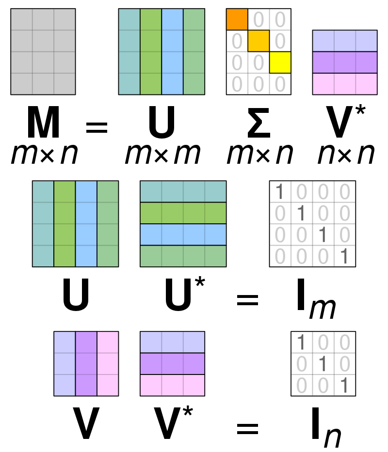
适用于m*n的矩阵，分解形式

$$ {\displaystyle A=UDV^{*}} $$

D是非负的对角阵，U和V是酉矩阵（实数上就是正交矩阵）

D的对角元称为A的奇异值

A的奇异值是唯一的，U和V不一定唯一

在有些地方把奇异值分解的形式写成

$$ {\displaystyle \ \mathbf {M} =\mathbf {U\Sigma V^{*}} \ } $$

其中，矩阵的大小为

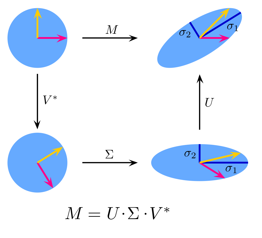
奇异值分解的几何意义是

对于M在空间上所做的变换，U将空间进行旋转，Σ将空间进行缩放，V*再将空间进行旋转，Σ的对角元就是缩放的比例

如果M的行列式是正的，那么U，V*可以都带反射（reflection）（就是将一张纸翻过来），或者都不带反射，如果M的行列式是负的，那么U或V*带反射

如果M不是方阵，假设是m*n的，几何意义可以看作是n维空间到m维空间的变换，U和V*分别作用于m维和n维空间，Σ除了对min(m,n)维空间进行缩放后，在其他维度要补0，以便后续的计算

Example

$$ \mathbf {M} ={\begin{bmatrix}1&0&0&0&2\\0&0&3&0&0\\0&0&0&0&0\\0&2&0&0&0\end{bmatrix}} $$

$$ {\displaystyle {\begin{aligned}\mathbf {U} &={\begin{bmatrix}\color {Green}0&\color {Blue}-1&\color {Cyan}0&\color {Emerald}0\\\color {Green}-1&\color {Blue}0&\color {Cyan}0&\color {Emerald}0\\\color {Green}0&\color {Blue}0&\color {Cyan}0&\color {Emerald}-1\\\color {Green}0&\color {Blue}0&\color {Cyan}-1&\color {Emerald}0\end{bmatrix}}\\[6pt]{\boldsymbol {\Sigma }}&={\begin{bmatrix}3&0&0&0&\color {Gray}{\mathit {0}}\\0&{\sqrt {5}}&0&0&\color {Gray}{\mathit {0}}\\0&0&2&0&\color {Gray}{\mathit {0}}\\0&0&0&\color {Red}\mathbf {0} &\color {Gray}{\mathit {0}}\end{bmatrix}}\\[6pt]\mathbf {V} ^{*}&={\begin{bmatrix}\color {Violet}0&\color {Violet}0&\color {Violet}-1&\color {Violet}0&\color {Violet}0\\\color {Plum}-{\sqrt {0.2}}&\color {Plum}0&\color {Plum}0&\color {Plum}0&\color {Plum}-{\sqrt {0.8}}\\\color {Magenta}0&\color {Magenta}-1&\color {Magenta}0&\color {Magenta}0&\color {Magenta}0\\\color {Orchid}0&\color {Orchid}0&\color {Orchid}0&\color {Orchid}1&\color {Orchid}0\\\color {Purple}-{\sqrt {0.8}}&\color {Purple}0&\color {Purple}0&\color {Purple}0&\color {Purple}{\sqrt {0.2}}\end{bmatrix}}\end{aligned}}} $$

另一个V*

$$ {\displaystyle \mathbf {V} ^{*}={\begin{bmatrix}\color {Violet}0&\color {Violet}1&\color {Violet}0&\color {Violet}0&\color {Violet}0\\\color {Plum}0&\color {Plum}0&\color {Plum}1&\color {Plum}0&\color {Plum}0\\\color {Magenta}{\sqrt {0.2}}&\color {Magenta}0&\color {Magenta}0&\color {Magenta}0&\color {Magenta}{\sqrt {0.8}}\\\color {Orchid}{\sqrt {0.4}}&\color {Orchid}0&\color {Orchid}0&\color {Orchid}{\sqrt {0.5}}&\color {Orchid}-{\sqrt {0.1}}\\\color {Purple}-{\sqrt {0.4}}&\color {Purple}0&\color {Purple}0&\color {Purple}{\sqrt {0.5}}&\color {Purple}{\sqrt {0.1}}\end{bmatrix}}} $$

SVD分解的过程参考此处

Schur complement

舒尔补的作用是将p+q维矩阵的求逆变成p维和q维矩阵的求逆，降低运算时间

SLAM和舒尔补

假设A、B、C、D矩阵为 p × p, p × q, q × p, q × q

$$ {\displaystyle M=\left[{\begin{matrix}A&B\\C&D\end{matrix}}\right]} $$

假设D是可逆的（即非奇异），则D在M中的舒尔补为

$$ {\displaystyle M/D:=A-BD^{-1}C} $$

假设A是可逆的，则A在M中的舒尔补为

$$ {\displaystyle M/A:=D-CA^{-1}B} $$

舒尔补在高斯消元中有用到，为了使M变成上三角矩阵，可以右乘一个下三角矩阵

$$ {\displaystyle {\begin{aligned}&M={\begin{bmatrix}A&B\\C&D\end{bmatrix}}\quad \to \quad {\begin{bmatrix}A&B\\C&D\end{bmatrix}}{\begin{bmatrix}I_{p}&0\\-D^{-1}C&I_{q}\end{bmatrix}}={\begin{bmatrix}A-BD^{-1}C&B\\0&D\end{bmatrix}}\end{aligned}}} $$

Ip是p阶单位阵，可以发现最后矩阵的左上角出现了D在M中的舒尔补

将这个结果左乘一个矩阵后转化为对角阵

$$ {\displaystyle {\begin{aligned}&{\begin{bmatrix}A-BD^{-1}C&B\\0&D\end{bmatrix}}\quad \to \quad {\begin{bmatrix}I_{p}&-BD^{-1}\\0&I_{q}\end{bmatrix}}{\begin{bmatrix}A-BD^{-1}C&B\\0&D\end{bmatrix}}={\begin{bmatrix}A-BD^{-1}C&0\\0&D\end{bmatrix}}\end{aligned}}} $$

由此可以引导出M的LDU分解

$$ {\displaystyle {\begin{aligned}M&={\begin{bmatrix}A&B\\C&D\end{bmatrix}}={\begin{bmatrix}I_{p}&BD^{-1}\\0&I_{q}\end{bmatrix}}{\begin{bmatrix}A-BD^{-1}C&0\\0&D\end{bmatrix}}{\begin{bmatrix}I_{p}&0\\D^{-1}C&I_{q}\end{bmatrix}}\end{aligned}}} $$

所以M的逆可以由D的逆和舒尔补的逆组成

$$ {\displaystyle {\begin{aligned}M^{-1}={\begin{bmatrix}A&B\\C&D\end{bmatrix}}^{-1}={}&\left({\begin{bmatrix}I_{p}&BD^{-1}\\0&I_{q}\end{bmatrix}}{\begin{bmatrix}A-BD^{-1}C&0\\0&D\end{bmatrix}}{\begin{bmatrix}I_{p}&0\\D^{-1}C&I_{q}\end{bmatrix}}\right)^{-1}\\={}&{\begin{bmatrix}I_{p}&0\\-D^{-1}C&I_{q}\end{bmatrix}}{\begin{bmatrix}\left(A-BD^{-1}C\right)^{-1}&0\\0&D^{-1}\end{bmatrix}}{\begin{bmatrix}I_{p}&-BD^{-1}\\0&I_{q}\end{bmatrix}}\\[4pt]={}&{\begin{bmatrix}\left(A-BD^{-1}C\right)^{-1}&-\left(A-BD^{-1}C\right)^{-1}BD^{-1}\\-D^{-1}C\left(A-BD^{-1}C\right)^{-1}&D^{-1}+D^{-1}C\left(A-BD^{-1}C\right)^{-1}BD^{-1}\end{bmatrix}}\\[4pt]={}&{\begin{bmatrix}\left(M/D\right)^{-1}&-\left(M/D\right)^{-1}BD^{-1}\\-D^{-1}C\left(M/D\right)^{-1}&D^{-1}+D^{-1}C\left(M/D\right)^{-1}BD^{-1}\end{bmatrix}}\end{aligned}}} $$

这是一种形式，可以交换A和D来推导出另一种形式

Properties

假设p和q都是1，AD-BC不为0

$$ M^{{-1}}={\frac {1}{AD-BC}}\left[{\begin{matrix}D&-B\\-C&A\end{matrix}}\right] $$

当A是可逆的，那么

$$ {\displaystyle {\begin{aligned}M&={\begin{bmatrix}A&B\\C&D\end{bmatrix}}={\begin{bmatrix}I_{p}&0\\CA^{-1}&I_{q}\end{bmatrix}}{\begin{bmatrix}A&0\\0&D-CA^{-1}B\end{bmatrix}}{\begin{bmatrix}I_{p}&A^{-1}B\\0&I_{q}\end{bmatrix}},\\[4pt]M^{-1}&={\begin{bmatrix}A^{-1}+A^{-1}B(M/A)^{-1}CA^{-1}&-A^{-1}B(M/A)^{-1}\\-(M/A)^{-1}CA^{-1}&(M/A)^{-1}\end{bmatrix}}\end{aligned}}} $$

当A（D）是可逆的，则

$$ {\displaystyle \det(M)=\det(A)\det \left(D-CA^{-1}B\right)}\\{\displaystyle \det(M)=\det(D)\det \left(A-BD^{-1}C\right)} $$

当D是可逆的，则

$$ {\displaystyle \operatorname {rank} (M)=\operatorname {rank} (D)+\operatorname {rank} \left(A-BD^{-1}C\right)} $$

Application to solving linear equations

假设要解这样的线性方程

$$ {\displaystyle {\begin{bmatrix}A&B\\C&D\end{bmatrix}}{\begin{bmatrix}x\\y\end{bmatrix}}={\begin{bmatrix}u\\v\end{bmatrix}}} $$

假设A是可逆的，可以得到

$$ {\displaystyle x=A^{-1}(u-By)} $$

将上式代入可以得到

$$ {\displaystyle \left(D-CA^{-1}B\right)y=v-CA^{-1}u} $$

定义A的舒尔补

$$ {\displaystyle S\ {\overset {\underset {\mathrm {def} }{}}{=}}\ D-CA^{-1}B} $$

x和y可以变成

$$ {\displaystyle y=S^{-1}\left(v-CA^{-1}u\right)} $$

$$ {\displaystyle x=\left(A^{-1}+A^{-1}BS^{-1}CA^{-1}\right)u-A^{-1}BS^{-1}v} $$

可以写成如下形式

$$ {\displaystyle {\begin{bmatrix}x\\y\end{bmatrix}}={\begin{bmatrix}A^{-1}+A^{-1}BS^{-1}CA^{-1}&-A^{-1}BS^{-1}\\-S^{-1}CA^{-1}&S^{-1}\end{bmatrix}}{\begin{bmatrix}u\\v\end{bmatrix}}} $$

大矩阵的逆可以分解成小矩阵的逆

$$ {\displaystyle {\begin{bmatrix}A&B\\C&D\end{bmatrix}}^{-1}={\begin{bmatrix}A^{-1}+A^{-1}BS^{-1}CA^{-1}&-A^{-1}BS^{-1}\\-S^{-1}CA^{-1}&S^{-1}\end{bmatrix}}={\begin{bmatrix}I_{p}&-A^{-1}B\\&I_{q}\end{bmatrix}}{\begin{bmatrix}A^{-1}&\\&S^{-1}\end{bmatrix}}{\begin{bmatrix}I_{p}&\\-CA^{-1}&I_{q}\end{bmatrix}}} $$

Something confusing

• 矩阵左乘一个行向量的几何意义

Reference

无水印的图来自wikipedia